Your business in 360°
Supply forecasting with Power BI: from data to purchase order

You can build a supply forecast in Power BI yourself, but a forecast line on its own is not enough. It becomes useful when sales history, stock levels and supplier orders sit in a single model, the data refreshes on its own, and the forecast turns into a specific order quantity for each item. For Rivilė and Finvalda users, what takes up most of the time is not the forecast itself but this data foundation. That is exactly what Analitika360 provides as ready-built Power BI report packages with automatic refresh.
In brief
- A supply forecast answers not the question of how much you will sell, but how much you need to order: forecast demand minus what you already have and what you have already ordered.
- You will need sales history by item and date, stock levels, reserved quantities, open supplier orders, delivery lead times and minimum order quantities.
- The line chart in Power BI Desktop has a built-in forecasting feature in which you set the period, seasonality and confidence interval. The order quantity is calculated by a DAX measure.
- A forecast is only as good as the freshness of its data, so the reports must refresh automatically, without manual exports to Excel.
- The Rivilė and Finvalda packages start at €59 a month, while a bespoke supply model is built as a custom project.
Contents
- What a supply forecast actually calculates
- What data you will need
- How to build a supply forecast in Power BI: 6 steps
- How to extend the forecast to fit your business
- A ready-made foundation for Rivilė and Finvalda users
- Our view
- FAQ
- Sources
What a supply forecast actually calculates
A sales forecast shows how many goods or raw materials you are likely to need. A supply forecast goes one step further: it compares that demand with what is already in the warehouse or on its way, and shows what is missing. If you would like to strengthen the sales side first, we cover it in more detail in our guide to sales forecasting with Power BI.
The simplified formula looks like this:
Order quantity = forecast demand + confirmed orders + safety stock − (stock on hand − reserved + on order from suppliers)

It is important to keep two signals apart here. Forecast demand is a statistical estimate based on history. Confirmed orders, such as a banquet or a wholesale customer’s order, are fact. If you mix them up, the forecast will either double-count quantities or miss a large order.
Example: chicken fillet for a restaurant chain
| Measure | Quantity, kg |
|---|---|
| Next week’s forecast (normal sales) | 420 |
| Confirmed banquet orders | 60 |
| Safety stock | 50 |
| Stock in the warehouse | 150 |
| Reserved for other sites | 20 |
| Already ordered from the supplier | 100 |
| Recommended order | 300 |
Calculation: 420 + 60 + 50 − (150 − 20 + 100) = 300 kg. If the supplier only accepts multiples of 25 kg, 300 kg works. If not, the quantity is rounded up to the nearest multiple.
What data you will need
Before building any visuals, it is worth agreeing on a minimum data set. This is enough for a first reliable forecast:
- Sales history by date, item and site or warehouse. In Rivilė and Finvalda, these are the lines of the sales documents.
- Stock levels by item and location. If you plan supply separately for each restaurant or warehouse, the location dimension must be kept throughout the model. This is also how the Microsoft Business Central inventory forecasting report works, analysing quantities by location, item and entry type.
- Reserved quantities and confirmed customer orders.
- Open supplier orders not yet delivered.
- Supplier terms: lead time in days, minimum order quantity, pack multiple. These are usually kept in Excel or a SharePoint list.
- Item groups, for assessing seasonality and trends at group level when an individual item’s history is too short.
Messy data should be fixed first where it affects the ordering decision: item codes, supplier records and stock levels. An item whose code is written differently in different warehouses turns into two separate items in the forecast.
How to build a supply forecast in Power BI: 6 steps
1. Connect and combine the sources
Power Query, Power BI’s data preparation tool, lets you import several sources and merge them on a shared key, such as the item code. A Microsoft tutorial in Lithuanian shows how product data from Excel is combined with order data and grouped by product and year.
This is where people most often get stuck: data from the accounting system has to be extracted, cleaned and kept continuously up to date. The Analitika360 packages move Rivilė and Finvalda data into a Power BI model automatically and let you connect additional sources such as Excel, SharePoint or logistics systems. You can read more about combining Rivilė and Excel data in this guide.
2. Organise the data model
The foundation consists of fact tables (sales, stock levels, supplier orders) and the dimensions that link them: a date table, items, locations and suppliers. A date table with no gaps is essential, because the forecasting feature and time comparisons rely on a continuous time axis.
A common mistake: months with no sales simply disappear from the data. The forecast then sees only the “good” months and overestimates demand. Missing periods must be zeros, not blanks.
3. Create a baseline forecast
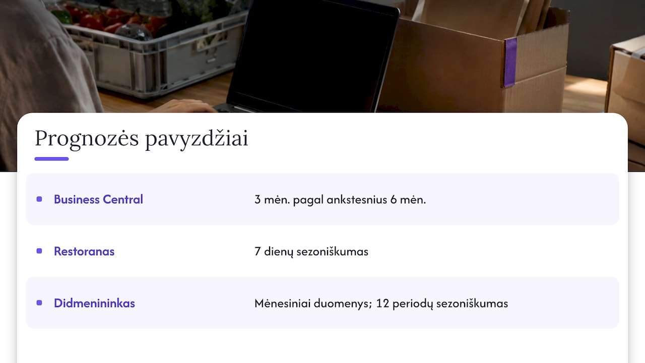
In a line chart with a date axis, open the Analytics pane and switch on Forecast. According to the Microsoft Learn description, Power BI Desktop lets you change the forecast length, seasonality, period and confidence interval. In the same Business Central example, quantities for the next 3 months are forecast from the previous 6 months, assuming monthly seasonality. These are the parameters of a specific example, not a rule for everyone.
In practice: for a restaurant whose turnover varies by day of the week, it makes sense to set seasonality to 7 days. For a wholesaler whose sales change with the seasons, monthly data and a seasonality of 12 periods will be a better fit.
4. Turn the forecast into an order quantity
The built-in forecast shows the trend on a chart, but the order quantity needs a DAX measure. DAX is Power BI’s formula language. A simplified example:
Rekomenduojamas užsakymas =
VAR Poreikis = [Prognozuojamas kiekis] + [Patvirtinti užsakymai] + [Saugos atsarga]
VAR Turima = [Likutis] - [Rezervuota] + [Užsakyta iš tiekėjų]
VAR Trukumas = Poreikis - Turima
VAR Kartotinis = MAX ( 'Tiekėjų sąlygos'[Kartotinis] )
RETURN
    IF ( Trukumas <= 0, 0, CEILING ( Trukumas, Kartotinis ) )
Here the forecast quantity can be calculated as a moving average of previous weeks, multiplied by a seasonality factor. The lead time determines the period over which demand is summed: if the supplier delivers within 10 days, demand is calculated at least 10 days ahead.
5. Automate the refresh
A forecast based on yesterday’s stock levels leads to the wrong order. When the data sources sit on a local server, a data gateway lets the Power BI service connect to them. We explain how it works in our Power BI data gateway guide. Analitika360 reports refresh without any further action from the user, so the purchasing manager or restaurant owner sees that day’s picture in the morning and no longer exports data by hand.
6. Check the forecast’s accuracy
One page of the report should show the forecast and the actuals side by side. A few measures are enough:
- WAPE (weighted absolute percentage error): the sum of all errors divided by total actual demand. It shows how far off the forecast is on average.
- Bias: whether the forecast is consistently too high or too low. A forecast that is consistently too high inflates stock and write-offs; one that is too low leads to shortages.
- Comparison with a simple method: whether your forecast is more accurate than “same as last week”. If it is not, the model needs reviewing.
Assess periods of zero demand separately, as they heavily distort percentage errors.
How to extend the forecast to fit your business
Once the baseline forecast is working, Power BI lets you adapt it to specific processes:
- Scenarios: parameter controls that let the purchasing manager change the growth rate, price or safety stock and immediately see the effect on the order and the margin.
- Promotions and events: a separate table of planned promotions or holidays that adjust demand.
- Cash flow: a large order means a large payment to the supplier. It is worth linking the supply forecast to a cash flow forecast so that the finance director can see when and how much cash will be needed.
- Sector specifics: for restaurants, ingredient turnover and write-offs matter; for logistics, lead times; for construction, material requirements by project stage.
A ready-made foundation for Rivilė and Finvalda users
Analitika360 Power BI report packages are built to analyse Rivilė and Finvalda data. They show sales, warehouse, revenue, cost, profit and debt indicators, refresh automatically and let you connect Excel, SharePoint, CRM or logistics sources. This is the same data foundation on which a supply forecast is built.
| Package | Price |
|---|---|
| Rivilė Basic | €59 a month |
| Rivilė PRO | €89 a month |
| Finvalda Basic | €59 a month |
| Finvalda PRO | €89 a month |
| Custom projects | €70 an hour |
A supply model with your supplier terms, scenarios and order calculation is tailored to the company’s processes and existing IT systems as a custom project. Finvalda users would do well to start with Finvalda warehouse reports.
Our view
Supply forecasts usually fail not because of the algorithm. They fail because data from the accounting system reaches the report too late, incomplete, or after being copied into Excel by hand.
That is why we start with the foundation: automatically refreshing Rivilė or Finvalda data in a single Power BI model alongside other sources. Once sales, stock levels and supplier orders are in one place, the forecast and the order quantity become an everyday working tool rather than a file rebuilt every month.
We tailor specific needs, such as ingredient planning for a restaurant or construction material requirements by project, to each company’s processes. This way the business makes decisions quickly and on the basis of facts.
Analitika360
FAQ
Can Power BI really forecast supply requirements?
Yes. The line chart in Power BI Desktop has a built-in forecasting feature with an adjustable period, seasonality and confidence interval. For the order quantity, which takes stock levels, reservations and supplier terms into account, additional DAX measures are created.
How much historical data do I need?
It depends on seasonality. In the Microsoft Business Central example, 3 months are forecast from the previous 6 months. If your sales vary strongly over the year, you will only see annual seasonality reliably with at least one or two years of history.
Can I use Rivilė or Finvalda data without manual exports?
Yes. Analitika360 packages move Rivilė and Finvalda data into Power BI and refresh it automatically. Additional sources, such as supplier terms in an Excel file or SharePoint list, can be connected to the same model.
How much does such a solution cost?
The Rivilė and Finvalda Basic packages cost €59 a month and the PRO packages €89 a month. A bespoke supply forecasting model is built as a custom project at €70 an hour.
Sources
Microsoft Learn: Inventory Forecasting (Power BI report), Business Central Microsoft Support: Learn to combine multiple data sources (Power Query)